
Without a doubt the Stochastic Oscillator is a universally used indicator. It uses such a simple yet powerful formula in order to detect rapid oversold and overbought conditions. This article discusses a certain strategy based on this indicator.
Coding the Stochastic Oscillator in Pine Script 🔗
The stochastic oscillator is a bounded technical indicator seeks to find oversold and overbought zones by incorporating the highs and lows using the normalization formula as shown below:
This means that at any time, it must be bounded between 0 and 100 as dictated by the mathematical formula above. We generally use the oscillator in a contrarian way where we use the concepts of oversold and overbought to describe certain extreme events.
An overbought level is an area where the market is perceived to be extremely bullish and is bound to consolidate, therefore giving us a bearish bias. An oversold level is an area where market is perceived to be extremely bearish and is bound to bounce, therefore giving us a bullish bias. Hence, the stochastic oscillator is a contrarian indicator that seeks to signal the expected reactions of extreme movements.
The answer to that is because we want to learn how to code all types of indicators from scratch in Pine Script so that we become fluent and comfortable back-testing and tweaking any strategy. By understanding how to code it, we are also able to code variations on the indicator such as the stochastic smoothing oscillator, an indicator discussed in previous articles.
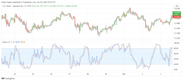
Generally, we smooth the oscillator with a 3-period moving average applied onto it. This can be seen in the above chart with the orange line following the stochastic in blue.
To code the oscillator, we first start by choosing the version of Pine Script, the official language of TradingView. In our case, we will choose the latest version. Then as we will create an indicator, we have to tell the program that we will do that by using the indicator() function. We will put two arguments inside, the title which we will call “Our Stochastic Oscillator” and the Boolean argument overlay. By putting false, we are telling the script that the oscillator will be in a different panel. If we were to create a moving average, we must put true.
// This source code is subject to the terms of the Mozilla Public License 2.0 at https://mozilla.org/MPL/2.0/
// © Sofien-Kaabar
// @version = 5
indicator("Our Stochastic Oscillator", overlay = false)
Next, we define the input values such as the lookback period, the oversold level, and the overbought level. We use the input() function to give us the opportunity to tweak these parameters on the settings directly from the chart. In other words, we do not have to code new parameters if we want to change them. The title is the name of the variable and the defval is the default value. In our case, it is 13, 20, and 80 as discussed previously.
lookback = input(title = 'Period', defval = 13)
oversold_level = input(title = 'Oversold', defval = 20)
overbought_level = input(title = 'Overbought', defval = 80)
Now, we will calculate the highest highs and the lowest lows in the lookback period so that we construct the stochastic formula. This is done by using the ta.highest() and ta.lowest() functions. Each require a lookback which in our case is the defined variable with a default value of 13.
// highest high
highest = ta.highest(high, lookback)// lowest low
lowest = ta.lowest(low, lookback)
The last step is applying the formula. This is simply done below where we define the stochastic_k (%K) followed by the stochastic_D (%D) which is the 3-period simple moving average of stochastic_k. The simple moving average is calculated using the ta.sma() function.
// stochastic oscillator
stochastic_K = ((close - lowest) / (highest - lowest)) * 100
stochastic_D = ta.sma(stochastic_K, 3)
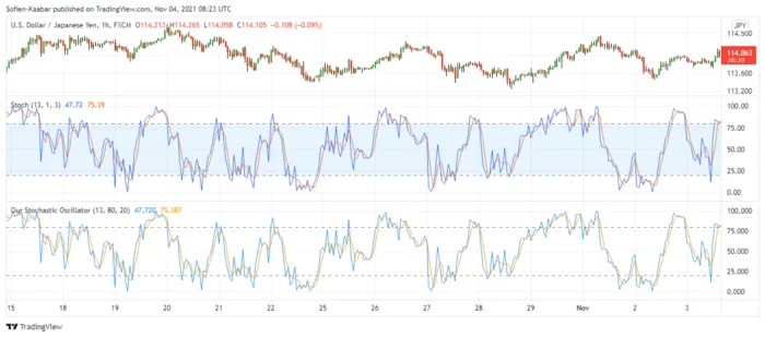
Let us plot what we have so far and compare it to the built-in stochastic oscillator script.
plot(stochastic_K)
plot(stochastic_D, color = color.orange)
hline(oversold_level)
hline(overbought_level)
// This source code is subject to the terms of the Mozilla Public License 2.0 at https://mozilla.org/MPL/2.0/
// © Sofien-Kaabar
// @version = 5
indicator("Our Stochastic Oscillator", overlay = false)lookback = input(title = 'Period', defval = 13)
oversold_level = input(title = 'Oversold', defval = 20)
overbought_level = input(title = 'Overbought', defval = 80)// highest high
highest = ta.highest(high, lookback)// lowest low
lowest = ta.lowest(low, lookback)// stochastic oscillator
stochastic_K = ((close - lowest) / (highest - lowest)) * 100
stochastic_D = ta.sma(stochastic_K, 3)plot(stochastic_K)
plot(stochastic_D, color = color.orange)
hline(oversold_level)
hline(overbought_level)
Coding and Analyzing the Strategy in Pine Script 🔗
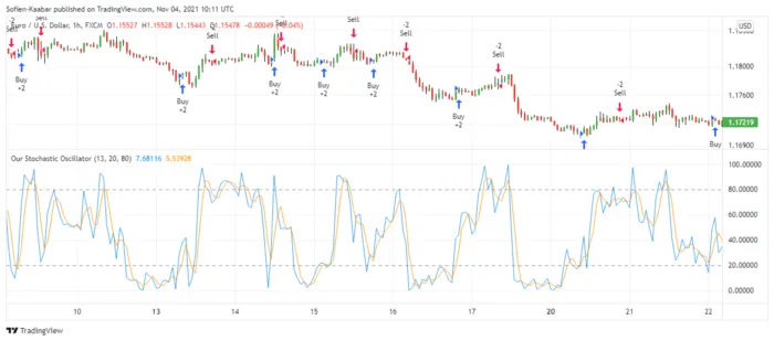
The strategy is pretty clear, we will initiate position based on the exit of extremes. Therefore, the trading conditions are:
- A buy (Long) signal is generated whenever the current 13-period stochastic oscillator is above 20 while the previous reading is below 20.
- A sell (Short) signal is generated whenever the current 13-period stochastic oscillator is below 80 while the previous reading is above 80.
Let us code the conditions of the signals first. When we use the stochastic_K[1] statement, it refers to the previous value of wherever we are now.
buy_signal  = stochastic_K > oversold_level and stochastic_K[1] < oversold_level
sell_signal = stochastic_K < overbought_level and stochastic_K[1] > overbought_level
Now, to simulate the orders, we use strategy.entry() built-in function which allows us to either go long or short whenever the signal is generated. The position is initiated at the opening price after the signal. (Which itself is generated at the close).
strategy.entry('Buy',  strategy.long,  when = buy_signal)
strategy.entry('Sell', strategy.short, when = sell_signal)
// This source code is subject to the terms of the Mozilla Public License 2.0 at https://mozilla.org/MPL/2.0/
// © Sofien-Kaabar
// @version=5

strategy("Our Stochastic Oscillator", overlay = false)lookback = input(title = 'Period', defval = 13)

oversold_level = input(title = 'Oversold', defval = 20)
overbought_level = input(title = 'Overbought', defval = 80)// highest high
highest = ta.highest(high, lookback)// lowest low
lowest = ta.lowest(low, lookback)// stochastic oscillator
stochastic_K = ((close - lowest) / (highest - lowest)) * 100
stochastic_D = ta.sma(stochastic_K, 3)plot(stochastic_K)

plot(stochastic_D, color = color.orange)
hline(oversold_level)
hline(overbought_level)buy_signal  = stochastic_K > oversold_level and stochastic_K[1] < oversold_level

sell_signal = stochastic_K < overbought_level and stochastic_K[1] > overbought_levelstrategy.entry('Buy',  strategy.long,  when = buy_signal)
strategy.entry('Sell', strategy.short, when = sell_signal)
Summary 🔗
To sum up, what I am trying to do is to simply contribute to the world of objective technical analysis which is promoting more transparent techniques and strategies that need to be back-tested before being implemented. This way, technical analysis will get rid of the bad reputation of being subjective and scientifically unfounded.